Detectors and DLVAs
What a Detector Log Video Amplifier Is
Power in, voltage out, compressed logarithmically. The specification that matters is the shape of the line, not a point on it.
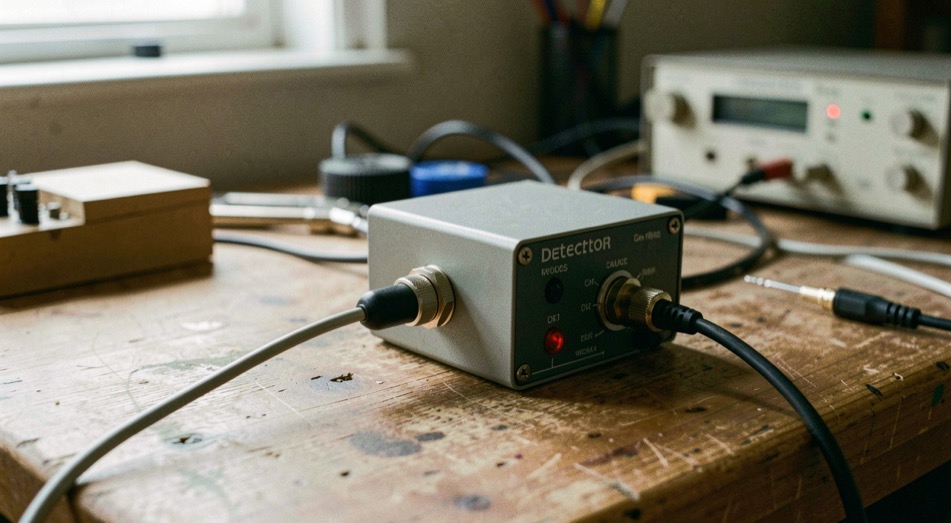
A detector log video amplifier is two functions graded as one part: a diode detector that turns microwave power into a video voltage, and a logarithmic video amplifier that compresses the result until the output follows the logarithm of input power. The pair is specified end to end, and its specification is a transfer curve, a slope in millivolts per decibel around an ideal straight line, never one number standing alone.
The diode first: voltage that tracks power
A detector converts RF power into a video voltage. At weak signal a diode operates in its quadratic regime: the output voltage is approximately proportional to input power, not to input voltage. That proportionality makes the front of the chain a power meter rather than a voltage meter, and it is conditional; the weak signal qualification is part of the behavior, not a footnote. The decibel scales mirror the split: 10 log10 for a power ratio, 20 log10 for a voltage ratio, both read in a 50 ohm system, the reference impedance of common coaxial microwave systems.
Why the range needs compressing
Power at a detector input does not arrive within a few percent of one level. It arrives across wide spans, and a voltage proportional to power would hand that span to the output unchanged: cover several factors of ten at the input and a proportional output covers the same factors of ten. The logarithmic stage exists to compress that span. Past it, the output is approximately proportional to the logarithm of input power, so equal steps of input in decibels give equal steps of output voltage. A constant figure in millivolts per decibel, the slope, is the direct product of that compression.
What does end to end mean on a datasheet?
The abbreviation names two components; the specification is one path. A detector log video amplifier is graded from its RF input to its video output, and the grading is a transfer curve: output voltage approximately equals the slope multiplied by input power in dBm, plus an intercept. The slope is stated in millivolts per decibel. The intercept is the reference point of the ideal straight line. Neither number works without the other, because the same intercept under a different slope describes a different line. Each term is defined once in the parameter index, and the point by point reading of the line is the subject of reading a transfer curve.
The chain, stage by stage
One housing does not merge the physics. Each stage fixes one property of the curve, and a specification that names the stage says where each number comes from.
| Stage | Role | What it fixes in the specification |
|---|---|---|
| Diode in the quadratic regime | Converts RF power to a video voltage proportional to power | The bottom of the usable range, where the weak signal condition holds |
| Logarithmic video amplifier | Makes the output follow the logarithm of input power | The compression, and the slope it delivers in mV/dB |
| The ideal straight line | Slope multiplied by input power in dBm, plus the intercept | The reference the real curve is graded against |
| Video bandwidth | Filters the video output | The pulse durations the output can reproduce, and the noise level behind sensitivity |
How much does a range number promise?
The measure of a logarithmic part is not its slope. It is the logging error: the deviation, in dB, between the real curve and the ideal straight line. Dynamic range is defined through that error, as the interval of input power over which the logging error stays inside a stated mask. The mask is the whole meaning. Two sheets quoting the same span under different masks are not comparable, and a range printed with no mask attached says nothing about the curve between its endpoints. Where the real curve departs from the line, power read off the ideal line is wrong by that departure.
Common mistakes
- Quoting a dynamic range without the mask it was measured under.
- Comparing two slopes in mV/dB while leaving the intercepts out of the comparison.
- Treating TSS as a fixed sensitivity number, detached from the video bandwidth in place during the measurement.
- Expecting the diode's quadratic proportionality across the whole input span; it is a weak signal property.
- Reading recovery time as a switching speed; it is a delay before a weak pulse can be measured correctly.
- Taking any single number as the specification; the part grades as a curve.
The two figures that move together
Sensitivity on short pulses is a property shared by two numbers. Tangential signal sensitivity, TSS, is the input level at which the top of the noise without signal and the bottom of the noise with signal become tangent on an oscilloscope. It is a visual, historical criterion: reproducible, but dependent on the observer and on the video bandwidth. Video bandwidth is the bandwidth of the output, and it sets the pulse durations the part can reproduce; widening it passes more noise and degrades TSS. The pair works as one tradeoff, examined in sensitivity and video bandwidth. Recovery time belongs to the same family: the delay after a strong pulse before a weak one can be measured correctly.
Before comparing two DLVA sheets
- Carry slope and intercept together as one straight line, not as two separate scores.
- Find the logging error mask before believing any dynamic range figure.
- Read TSS with the video bandwidth it was measured at, never alone.
- Match the video bandwidth to the shortest pulse to reproduce, not the longest.
- Check the recovery time condition: which strong pulse came before the weak one being measured.
- Confirm the levels are quoted in the same 50 ohm system as the rest of the bench.
A datasheet of this kind reads backward. Find the mask behind the dynamic range, then the video bandwidth behind the sensitivity figure, then the intercept behind the slope. A part specified as a curve is compared as a curve, and the comparison starts with the conditions, not with the headline span.