Detectors and DLVAs
Reading a Log Detector Transfer Curve
Dynamic range without a logging error limit is not a specification. This is how the two are read together.
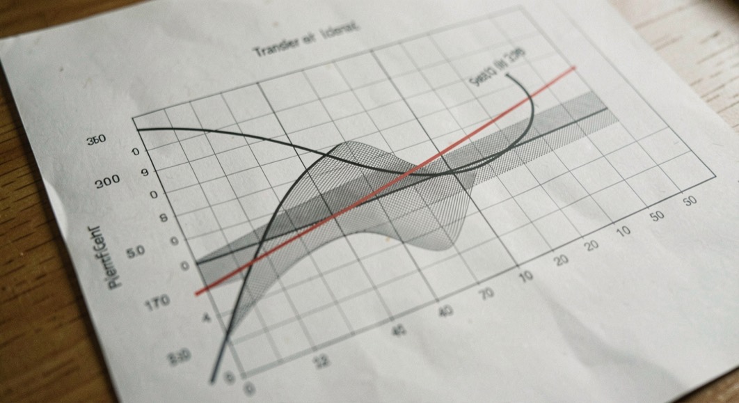
A log detector is not specified by one number. It is specified by a transfer curve, and reading that curve comes down to three quantities: a slope in millivolts per dB, an intercept, and a logging error in dB. The slope and the intercept describe an ideal straight line. The logging error says how far the real curve departs from that line, and the rest of the page, dynamic range included, is a statement about the size of that departure.
The dB is what makes the line straight
The mechanism starts with the detector. A detector converts RF power into a video voltage, and on its own, in the low signal regime, a diode detector is quadratic: its output voltage approximately follows the input power. A logarithmic video amplifier does the compressing. It drives its output to follow the logarithm of input power, which folds a very wide power span into a workable voltage swing. A detector log video amplifier chains the two functions and is specified end to end.
The straightness is a property of the axes. A decibel is a logarithm of a power ratio, dB = 10 log10(P2/P1), so a ratio of 1000 to 1 is 30 dB. Written in dBm, input power becomes an additive scale, and an output that follows the logarithm of power draws an approximately straight line against it.
What do the slope and the intercept fix?
The ideal line is written Vout ≈ slope × Pin(dBm) + intercept. The slope, in millivolts per dB, fixes how many millivolts the output climbs for each dB of input. The intercept fixes the reference point the ideal line is drawn through. Two parts with the same slope and different intercepts sit offset in voltage at the same input. Two parts with different slopes fan apart as the input rises, agreeing near one end of the span and disagreeing at the other.
The two figures are read together, and the arithmetic is worth doing once on paper. A slope of 10 mV/dB moves an output 600 mV across a 60 dB span. That is arithmetic on the definition, nothing more; the slope a real part delivers belongs to the part.
Where is the logging error largest?
The logging error, also called log linearity, is the deviation in dB between the real curve and the ideal straight line. It is the grade of a logarithmic response, because it describes the gap the reading actually crosses. It is not a single number either. It belongs to the whole curve, and where a range has been stated as wide as its limit allows, the deviation is at its largest at the two ends. That is not a separate observation: the range ends where the deviation reaches the limit it was promised to stay inside.
A page that prints one error figure for the whole range has flattened a curve into a value. What span that value was read over is the question to bring to it.
A dynamic range is a claim about an error budget
That is what the dynamic range column states: the interval of input power over which the logging error stays inside the stated template. The range and the template are one specification, not two. A range is a different claim at a tight template than at a loose one, and a range quoted with no template at all is not conservative. It is unreadable, and it invites the assumption that the error is uniform across the span, which the definition denies.
How the stages ahead of the curve shape what it receives is taken apart in the DLVA primer.
Before a range is read as a number
- Find the logging error limit, in dB, that the range is stated against.
- Confirm that the limit and the interval cover the same input span.
- Read the slope and the intercept as two separate figures; neither substitutes for the other.
- Work the slope arithmetic only once the span is known.
- Treat a range with no attached template as a headline, not a measurement.
The quantities, their units, and what each one fixes
Each figure on the page fixes one thing. Keeping them distinct is most of the work of reading the page.
| Quantity | Unit | What it fixes |
|---|---|---|
| Slope | mV/dB | How many millivolts the output climbs per dB of input |
| Intercept | mV | The reference point the ideal straight line is drawn through |
| Logging error | dB | How far the real curve departs from that line |
| Dynamic range | dB of input span | The interval over which the error stays inside the stated template |
| TSS | dBm | The input level at which the two noise edges become tangent |
| Video bandwidth | Hz | The shortest pulse the output reproduces, and how much noise it carries |
| Recovery time | s | How long a strong pulse blocks a weak one from being measured correctly |
Why do TSS and video bandwidth travel together?
TSS, tangential signal sensitivity, is the input level at which the top of the noise without signal and the bottom of the noise with signal become tangent on an oscilloscope. It is a visual criterion with a history: reproducible, but dependent on the observer and on the video bandwidth. The video bandwidth is the bandwidth of the output, and it fixes the shortest pulse the output can reproduce. Widening it passes more noise, and that noise degrades the TSS figure. One compromise, read from both ends; a sensitivity figure quoted without its video bandwidth is half a specification. The trade is set out further under sensitivity and video bandwidth.
Recovery time completes the set. It is the delay after a strong pulse before the detector can measure a weak one correctly, so a small signal arriving close behind a large one is not read by the same rule as a small signal arriving in the quiet.
Common mistakes
- Quoting a dynamic range with no logging error limit attached to it.
- Assuming the error is uniform across the range when it is largest at the ends.
- Reading a single error figure as if it described the whole curve rather than the span it was taken over.
- Taking a TSS figure without the video bandwidth it was read at.
- Comparing two sensitivity figures quoted at different video bandwidths.
- Measuring a weak pulse right after a strong one and carrying the number over as if the bench had been quiet.
The check is small enough to repeat on every sheet of this kind. Find the logging error limit first and write it beside the range before anything else on the page is read; find the video bandwidth and write it beside the sensitivity figure. Where a limit is missing, leave the column unresolved and ask for the error curve instead of the range.